3 General Ensemble Properties
The results of this chapter can be reproduced with the following Jupyter notebook: https://github.com/re-models/re-technical-report/blob/main/notebooks/chapter_general-props.ipynb.
Before analyzing how the model variants perform with regard to the described performance criteria, we will analyze some basic features of model runs that help us understand the model better. The resulting insights will (hopefully) help to understand and interpret some of the results, we will present in subsequent chapters.
In particular, we assess the overall length of processes, the (mean) step length of commitments adjustments steps, properties of global optima and the extent of branching.
Here and in the following chapters, we will assess different properties of model runs and their dependence (mainly) on the chosen model variant, the selection of \(\alpha\) weights and the size of the sentence pool. Admittedly, other dimensions as, for instance, properties of the dialectical structures (such as inferential density) are also interesting as independent variables to assess the performance of the different models. However, we had to confine the analysis to some extent and regard the chosen dimensions as particularly important.
Since we want to compare the performance of different model variants, we have, of course, to vary the model. The variation of \(\alpha\)-weights is important since the modeler has to choose a particular set of \(\alpha\)-weights in a specific context. It is therefore not enough to know how the different models compare to each other on average (with respect to \(\alpha\)-weights) but important to compare them within different confined spectra of \(\alpha\)-weight configurations. The dependence on the size of the sentence pool is motivated by the practical restrictions to use semi-globally optimizing model variants. Due to computational complexity the use of semi-globally optizing models is feasible for small sentence pools only. However, these small sentence pools are too small to model reflective equilibration of actual real-world debates.1 Accordingly, we are confined to use locally optimizing models in these cases. It is, therefore, of particular interest whether the observations of this ensemble study can be generalised to larger sentence pools.
3.1 Process Length and Step Length
In the following, we understand process length (\(l_p\)) as the number of theories and commitment sets in the evolution \(e\) of the epistemic state, including the initial and final state.
\[ \mathcal{C}_0 \rightarrow \mathcal{T}_0 \rightarrow \mathcal{C}_1 \rightarrow \mathcal{T}_1 \rightarrow \dots \rightarrow \mathcal{T}_{final} \rightarrow \mathcal{C}_{final} \]
In other words, if \((\mathcal{T}_{0}, \mathcal{C}_{0})\) is the initial state and \((\mathcal{T}_{m}, \mathcal{C}_{m})\) the fixed-point state, \(l_p(e)=2(m+1)\). An equilibration process reaches a fixed point if the newly chosen theory and commitments set are identical to the previous epistemic state—that is, if \((\mathcal{T}_{i+1}, \mathcal{C}_{i+1})=(\mathcal{T}_{i}, \mathcal{C}_{i})\) (Beisbart, Betz, and Brun 2021, 466). Therefore, the minimal length of a process is \(4\). In such a case, the achievement of initial commitments and the first chosen theory cannot be further improved. Accordingly, the initial commitments are also the final commitments.
Figure 3.1 shows the distribution of process lengths, and Figure 3.2 shows the mean process length (and its standard deviation) for the different model variants dependent on the size of the sentence pool (\(2n\)) over all branches.
Note that Figure 3.1 counts branches of a particular length for each model. One simulation setup can result in different branches if the adjustment of commitments or theories is underdetermined. Additionally, the number of branches for a specific simulation setup can vary between different models. Consequently, the overall number of branches per model can differ. This, in turn, explains why the sum of bars varies between the subfigures of Figure 3.1 (see Section 3.3 for details).
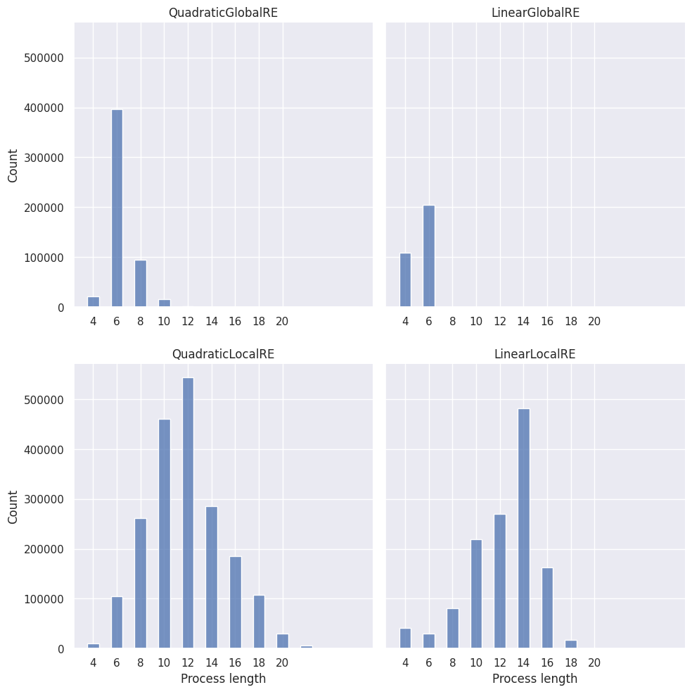
The first interesting observation is that the semi-globally optimizing models (QuadraticGlobalRE and LinearGlobalRE) reach their fixed points quickly. Often, they adjust their commitments only once (\(l_p(e)=6\)); the linear model variant (LinearGlobalRE) will sometimes not even adjust the initial commitments of processes (\(l_p(e)=4\)). In contrast, the locally optimizing models (QuardraticLocalRE and LinearLocalRE) need significantly more adjustment steps. This difference is expected if we assume that local and global optima commitments are not often in the \(1\)-neighbourhood of initial commitments (see Figure 3.4 and Figure 3.9). Under this assumption, the locally searching models will need more than one adjustment step to reach a global or local optimum.
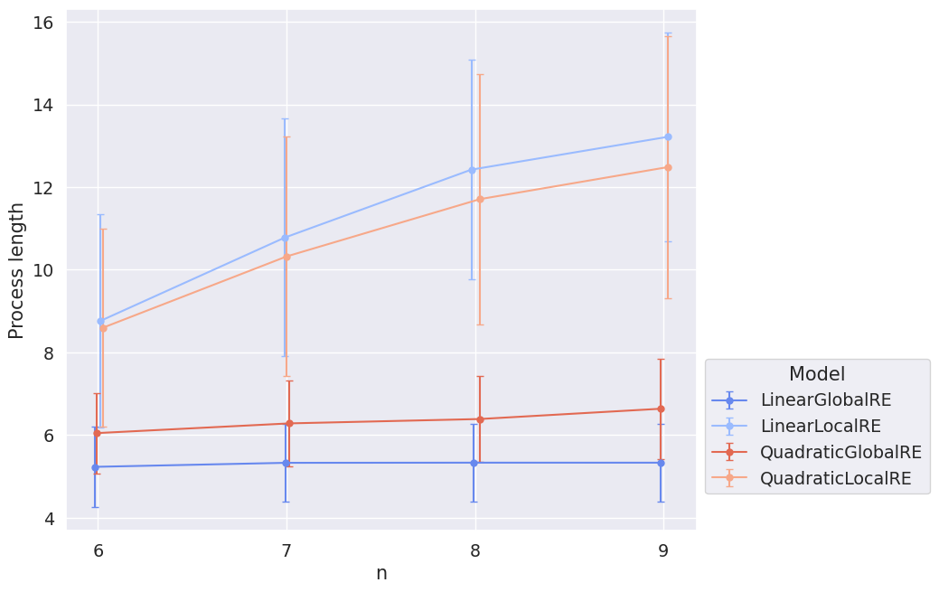
Additionally, the models QuardraticLocalRE and LinearLocalRE have a much larger variance in process lengths than the models QuadraticGlobalRE and LinearGlobalRE.
A third observation concerns the difference in process lengths between semi-globally and locally optimizing models in terms of their dependence on the sentence pool. Figure 3.2 suggests that the process length of locally optimizing models increases with the size of the sentence pool. The semi-globally optimizing models lack such a dependence on the sentence pool size.
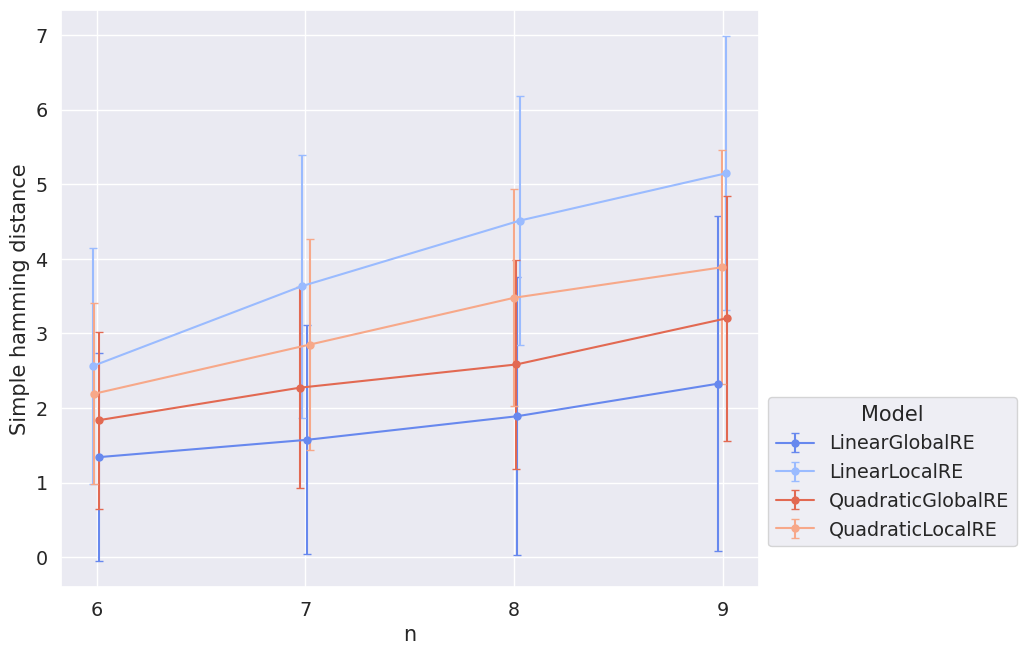
A possible explanation is motivated by analyzing the step length during the adjustment of commitments. Figure 3.3 shows the mean distance between adjacent commitments sets in the evolution of epistemic states over all branches. For simplicity, we measure the distance between two commitment sets by their simple Hamming distance, defined as the number of sentences not shared by both sets. For example, the simple Hamming distance between the commitments sets \(\{s_1,s_2\}\) and \(\{s_2,s_3\}\) is \(2\) since there are two sentences (\(s_1\) and \(s_3\)) not shared by both sets.
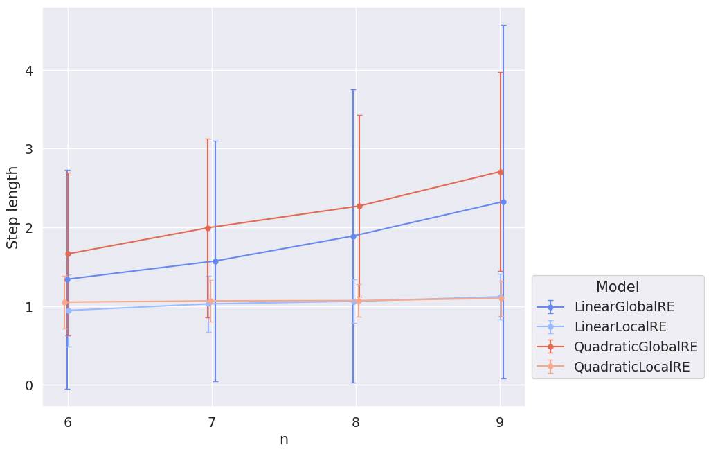
Unsurprisingly, the locally optimizing models have roughly a mean step length of \(1\) since they are confined in their choice of new commitments to the \(1\)-neighbourhood.2 In contrast, the semi-globally optimizing models take bigger leaps with an increasing sentence pool size. Figure 3.4 shows why: With the increasing size of the sentence pool, the mean distance between initial commitments and fixed-point commitments increases. In other words, RE processes must overcome larger distances to reach their final states. Semi-globally optimizing models can walk this distance with fewer steps (Figure 3.2) since they can take comparably large steps (Figure 3.3). Locally optimizing models are confined to small steps (Figure 3.3) and, thus, have to take more steps (Figure 3.2).
3.2 Global Optima
Global optima are fully determined by the achievement function of the RE model. Accordingly, global optima might differ between the linear and quadratic model variants but do not depend on whether the RE process is based on a local or semi-global optimization. In the following, we will therefore summarize analysis results with respect to global optima for linear models under the heading LinearRE and for quadratic models under the heading QuadraticRE.3
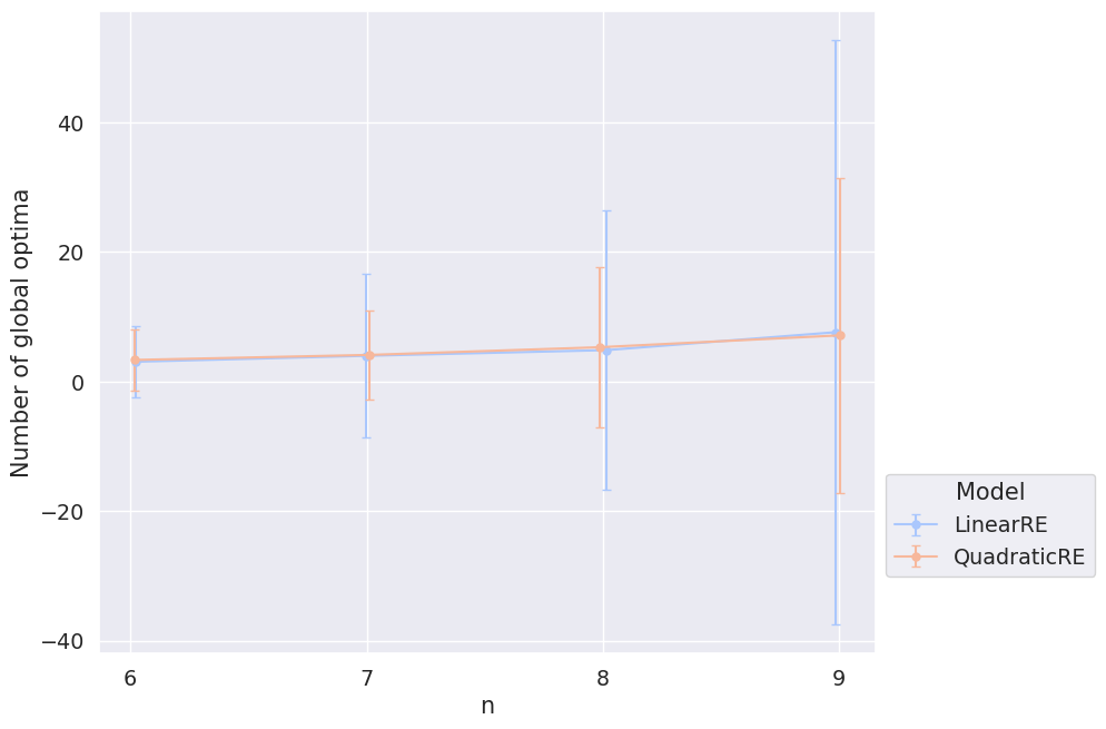
The mean number of global optima does not differ significantly between linear and quadratic models (\(5\pm 26\) vs. \(5\pm 14\)) and does not depend on the size of the sentence pool (see Figure 3.5).
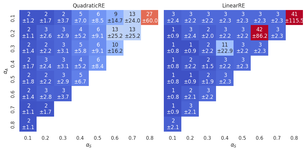
However, the heatmap in Figure 3.6 shows an interesting dependence on the \(\alpha\)-weights.
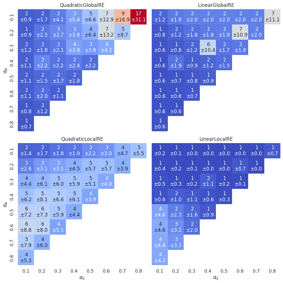
Here and in the following chapters, we will often rely on such heatmaps. Let us therefore provide some clarifications of their interpretation. If we are interested in visualising the dependence on \(\alpha\)-weight configurations (i.e., a specific triples of \(\alpha_A\), \(\alpha_F\) and \(\alpha_S\)), it is sufficient to use two dimensions (\(\alpha_A\) and \(\alpha_S\) in our case) since the three weights \(\alpha_A\), \(\alpha_F\) and \(\alpha_S\) are not independent. The diagonals in these heatmaps from southwest to northeast are isolines for the faithfulness weight (\(\alpha_F\)). In the following, we will refer to specific cells in these heatmaps in the typical \((x,y)\) fashion. For instance, we will call the cell with \(\alpha_S=0.5\) and \(\alpha_A=0.2\) the \((0.5,0.2)\) cell.
Now, let’s come back to Figure 3.6. For each simulation setup there is not necessarily one global optimum. Instead, there can be multiple global optima. Each cell in the heatmap provides for a specific \(\alpha\)-weight configuration the mean number of global optima (over all simulation setups with this \(\alpha\)-weight configuration). For the quadratic models, the number of global optima (and its variance) increases with an increase in \(\alpha_S\). For the linear models, on the other hand, the number of global optima is comparably low (\(1-3\)) in all cells with the exception of the three islands \((0.4,0.3)\), \((0.6,0.2)\) and \((0.8,0.1)\). These cells are characterised by \(\alpha_F = \alpha_A\). For linear models, there are more ties in the achievement function under these conditions (see Appendix A), which results in an increase in global optima.
Besides analysing the number of global optima, it is helpful to get a preliminary grasp on some topological properties of global optima. How are the commitments of global optima distributed over the space of all minimally consistent commitments? Are they located in a dense way to each other, or are they widely distributed in the whole space? What is their distance from initial commitments?
Figure 3.7 and Figure 3.8 depict the mean distance of global-optimum commitments in dependence of the sentence pool’s size and \(\alpha_F\). We calculated for each configuration setup that has more than one global optimum the mean (simple Hamming) distance between global-optimum commitments and took the average of these means with respect to different ensemble properties. The share of configuration setups that have more than one global optimum is \(0.58\) over all models, \(0.54\) for linear models and \(0.62\) for quadratic models.4
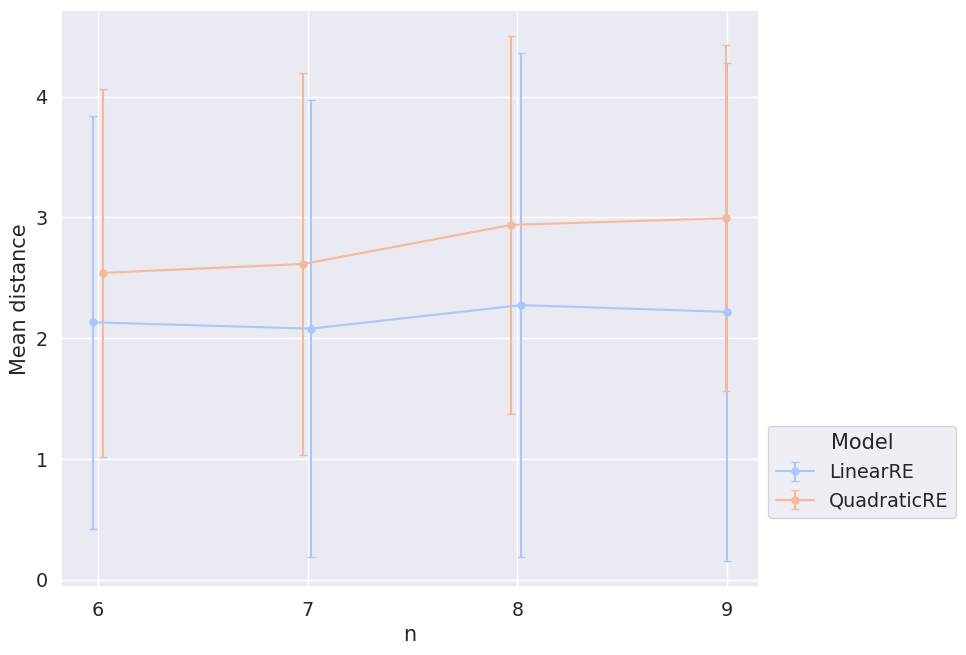
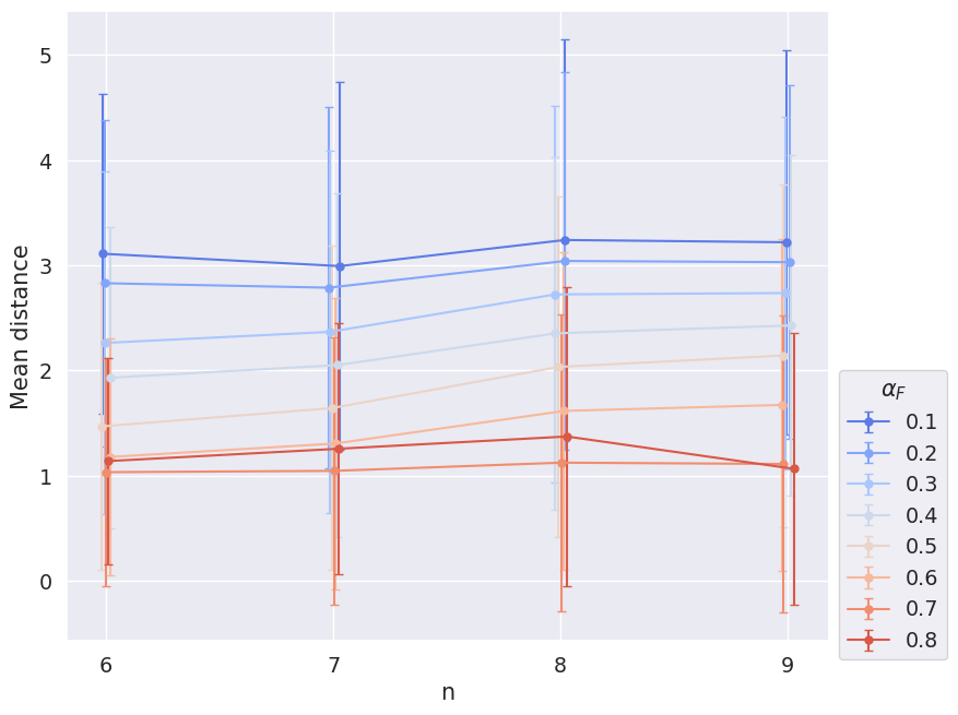
Figure 3.9 and Figure 3.10, one the other hand, depict the mean distance between initial commitments and global-optimum commitments. For that, we calculated for each simulation setup the mean (simple Hamming) distance between initial commitments and all global-optimum commitments of the simulation setup and, again, took the average of these means with respect to different ensemble properties.
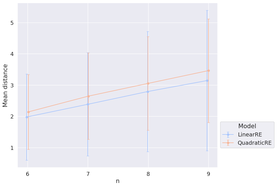
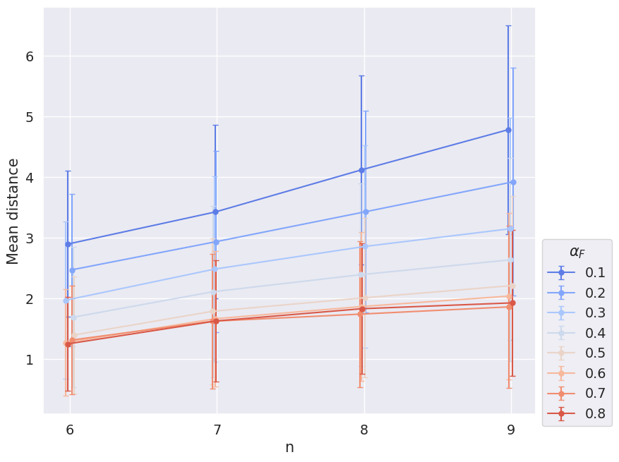
Figure 3.7 and Figure 3.9 are hard to interpret. The mean distance of global optima does not seem to depend on the size of the sentence pool; the mean distance of initial commitments and global-optimum commitments might increase with the size of the sentence pool. However, without an additional consideration of larger sentence pools, we cannot draw these conclusions with certainty due to the large variance.
Figure 3.8 and Figure 3.10, one the other hand, show that the mean distance of initial commitments and global-optimum commitments as well as the mean distance between global-optimum commitments depend on \(\alpha_F\). The smaller \(\alpha_F\), the larger the distance. This result is not suprising. The weight \(\alpha_F\) determines the extent to what final commitments should resemble initial commitments. You can think of \(\alpha_F\) as the magnitude of an attractive force that pulls the commitments of the epistemic state to the initial commitments. Accordingly, if \(\alpha_F\) gets smaller, global optima and fixed points will be distributed more widerspread in the space of epistemic states.
3.3 Branching
The choice of a new theory (or a new set of commitments respectively) is underdetermined if there are different candidate theories (or commitment sets) that maximize the achievement of the accordingly adjusted epistemic state. In such a case, the model randomly chooses the new epistemic state. The model we use is able to track all these different branches to assess the degree of this type of underdetermination and to determine all possible fixed points for each configuration setup.
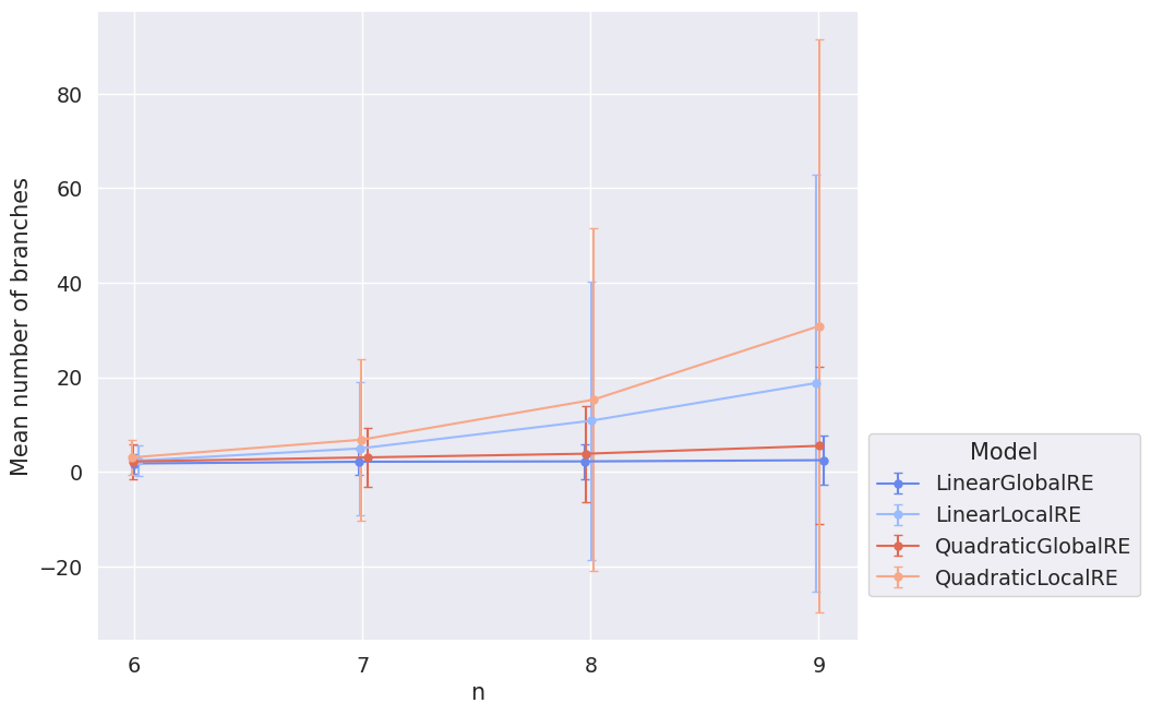
Figure 3.11 shows the mean number of branches with their dependence on the model and sentence pool. It suggests that branching is more prevalent in locally optimizing models. The large variance can be partly explained by the heat maps in Figure 3.12, which depict mean values (and standard deviations) for different weight combinations.
For LinearGlobalRE there are, again, islands with many branches (the cells \((0.4,0.3)\), \((0.6,0.2)\) and \((0.8,0.1)\)) which are characterised by \(\alpha_F = \alpha_A\). The high number of branches correlates with a high number of fixed points (compare Figure 3.13) and a high number of global optima within these cells (compare Figure 3.6). We might, therefore, hypothesize that the model produces a high number of branches in these cells due to the high number of global optima.5
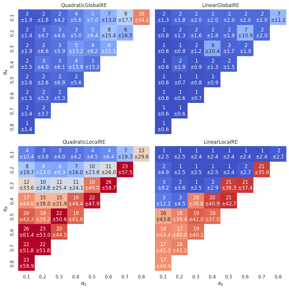
Interestingly, the identified hotspots of branches (and fixed points) for the LinearGlobalRE model are not reproduced by its locally optimizing cousin. This suggests that the LinearLocalRE model will perform worse than the LinearGlobalRE model to reach the increased amount of global optima.6
The “\(\alpha_F=\alpha_A\)”-line is, however, also relevant for the LinearLocalRE model. Above that line, branching is comparably low (roughly \(1-3\)) and below that line comparably high (with a high variance). The high number of branches does, however, not correlate with a high number of fixed points (see Figure 3.13). In other words, a lot of these branches end up in the same fixed point. This behaviour is to some extent even observable in the QuadraticLocalRE model.
Note/link about Andreas’ modelling of Tanja’s reconstruction.↩︎
The mean distance is, for some cases, slightly greater than \(1\), which can be simply explained: The definition of the \(1\)-neighbourhood is based on another Hamming distance than the one used here. In particular, there are sentence sets in the \(1\)-neighbourhood of a sentence set whose simple Hamming distance is greater than \(1\). For instance, the set \(\mathcal{C}_1=\{s_1, \neg s_2\}\) is in the \(1\)-neighbourhood of the sentence set \(\mathcal{C}_2=\{s_1,s_2\}\) since it only needs an attitude change towards one sentence (i.e., an attitude change towards \(s_2\) from rejection to acceptance). However, the simple Hamming distance is \(2\) since both \(s_2\) and \(\neg s_2\) are not shared by \(\mathcal{C}_1\) and \(\mathcal{C}_2\).↩︎
In our data set, the analysis results might differ between semi-globally and locally optimizing models, which is, however, an artifact of the difference in interrupted model runs (i.e., model runs that could not properly end (see Section 2.4)). For the subsequent analysis of global optima, we rely on the model results of
QuadraticGlobalREandLinearGlobalREsince they had fewer interrupted model runs.↩︎Note that global optima a process-independent. Hence, semi-globally and locally optimizing models do not differ with respect to their global optima.↩︎
In Chapter 4, we will analyze to what extent the model is able to reach these global optima. The numbers (\(7/8/8\) branches and fixed points and \(11/32/25\) global optima) suggest that the number of fixed points are nevertheless not enough to reach all these global optima (see, e.g., Figure 4.6 and Figure 4.14 in Chapter 4).↩︎
A hypothesis we will scrutinize in Chapter 4 (see, e.g., Figure 4.6 and Figure 4.14).↩︎